| Page |
|
© Peter Broadfoot 2008
Histograms
Exercise 4 – Frequency Polygon
a)
Is the data continuous or discrete?
Time is a continuous variable.
b)
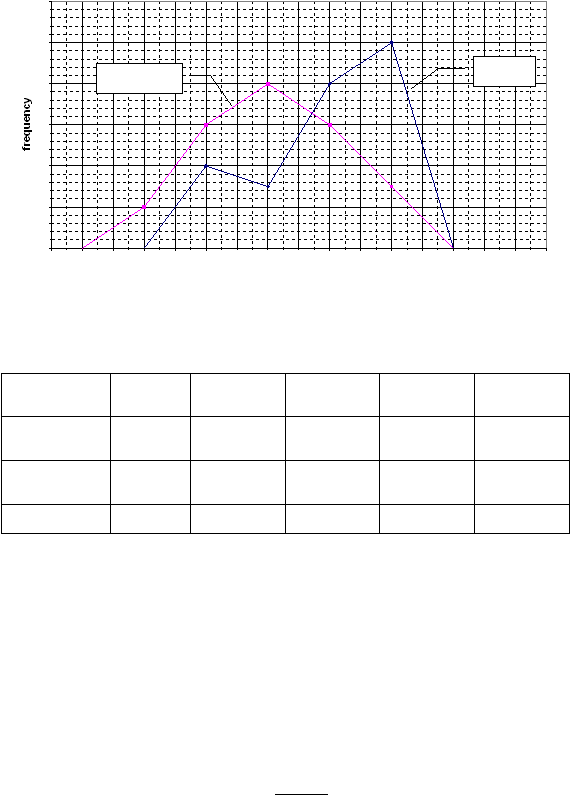
On (a copy of) the grid provided, draw separate frequency polygons for the men and the
women. Label the diagram fully.
Comparison: Times to Run a Race
0
2
4
6
8
10
12
20
25
30
35
40
45
50
55
60
65
70
75
80
85
90
95
100
Time (minutes)
This frequency diagram is based on the table of data given in the question, shown below
with the mid-points included. Check that you plotted your diagram at the mid-points.
Time
(minutes)
30≤t<40
40≤t<50
50≤t<60
60≤t<70
70≤t<80
Frequency:
men
0
4
3
8
10
Frequency:
women
2
6
8
6
3
Mid-point
35
45
55
65
75
Exercise 5 – Reading a Histogram
The question states:
For the histogram above, each 1cm square represents 2.5 items of data. Calculate the
number of items that weigh between 4.5 and 6kg.
The histogram has two classes between 4.5 and 6kg. The areas are 2 and 1.6cm^2. The
combined area is 3.6cm^2.
Therefore number of items
= number per square cm × area in cm^2.
= 2.5 × 3.6 = 9 items
Men
Women